Morphometric Characterisation of Root-Knot Nematode Populations from Three Regions in Ghana
Article information
Abstract
Tomato (Solanum lycopersicum) production in Ghana is limited by the root-knot nematode (Meloidogyne incognita, and yield losses over 70% have been experienced in farmer fields. Major management strategies of the root-knot nematode (RKN), such as rotation and nematicide application, and crop rotation are either little efficient and harmful to environments, with high control cost, respectively. Therefore, this study aims to examine morphometric variations of RKN populations in Ghana, using principal component analysis (PCA), of which the information can be utilized for the development of tomato cultivars resistant to RKN. Ninety (90) second-stage juveniles (J2) and 16 adult males of M. incognita were morphometrically characterized. Six and five morphometric variables were measured for adult males and second-stage juveniles (J2) respectively. Morphological measurements showed differences among the adult males and second-stage juveniles (J2). A plot of PC1 and PC2 for M. incognita male populations showed clustering into three main groups. Populations from Asuosu and Afrancho (Group I) were more closely related compared to populations from Tuobodom and Vea (Group II). There was however a single nematode from Afrancho (AF4) that fell into Group III. Biplots for male populations indicate, body length, DEGO, greatest body width, and gubernaculum length serving as variables distinguishing Group 1 and Group 2 populations. These same groupings from the PCA were reflected in the dendogram generated using Agglomerative Hierarchical Clustering (AHC). This study provides the first report on morphometric characterisation of M. incognita male and juvenile populations in Ghana showing significant morphological variation.
Body
Tomato (Solanum lycopersicum L.) is consumed worldwide and second to potato in terms of production (FAO, 2013). The crop serves as a vegetable crop in Ghana making up about 38% of total vegetable expenditure annually (Wolff, 1999). Cultivation of tomato has been an important economic activity in Ghana, especially in the Upper East, BrongAhafo and Ashanti regions with estimates up to 7.5 metric tonnes per hectare (Robinson and Kolavali, 2010). Ghana is one of the largest importer of tomato paste in the world with an average consumption rate of 25,000 metric tonnes per annum which is about $25 million (Aryeetey, 2006).
Root-knot nematodes (RKN) cause significant economic yield losses in tomato production in numerous areas of the world (Agrios, 2005). Four nematode species (Meloidogyne incognita, M. javanica, M. arenaria and M. hapla) are the most important nematode pests in tomatoes fields (Jacquet, 2005; Perry and Moens, 2009). The first three species are widely distributed in the warmer tropical regions of the world, however, M. hapla is more prevalent in the temperate regions (Naz et al., 2012).
Studies have showed that, M. incognita are present in Ghana and are a limiting factor in tomato production. Tomato yield losses of between 73% and 100% caused by M. incognita have been reported in the Guinea savannah zone of the country (Hemeng, 1981). A survey conducted in Ghana identified M. incognita as the most abundant nematode species in tomato fields (Osei et al., 2012).
Management of this devastating pest is of prime importance because; most of the tomato cultivars being grown by farmers in Ghana are susceptible to this nematode. Crop rotation and use of appropriate nematicides are the most common means employed in the control of nematodes, however, due to health, environmental and cost concerns, nematicidal use is not a desirable choice. Host plant resistance may also be applied to reduce populations if these pests are found to be uniform in a field, however, if these populations are mixed, then differing host-plant resistance approaches for their control might be essential; hence more explicit studies will need to be developed. Knowledge on variability among different geographical populations therefore becomes essential for the development of suitable control strategies.
Identification of variability in Meloidogyne spp. has been through morphometric characterization of populations (Eisenback, 1985; Hewlett and Tarjan, 1983; Jepson, 1983, 1987; Karssen, 2002; Kaur and Attri, 2013). Kaur and Attri (2013) conducted morphometric characterization of M. incognita from different host plants in four districts of Punjab, India and this showed significant variation among the populations.
In Ghana, information pertaining to morphological and morphometric features of Ghanaian populations of M. incognita has been little documented. Therefore, a morphological diversity study was conducted among field populations of M. incognita from three major tomato production regions (Ashanti, BrongAhafo, and Upper East) in Ghana to: i. Characterize M. incognita populations (juveniles and males) based on morphometric features ii. Identify the important morphometric characters in discriminating among the populations through Principal Component Analysis (PCA).
Materials and Methods
Sampling procedures
Sampling was carried out during the tomato-growing season (November, 2014), in nine main tomato-growing areas in three regions (Ashanti, BrongAhafo, and Upper East), which were Afrancho (AF), Akumadan (AK) and Asuosu (AS) in Ashanti region, Toubodom (TB), Techimantia (TCH) and Tanoso (TA) in BrongAhafo region and Tono (TO), Pwalugu (P) and Vea (V) in Upper East region. Two farms from each locality were randomly selected for soil and root sampling. Soil samples were randomly collected from the fields. A soil sample of about 1 kg was composed of ten randomized samples obtained at a depth of 15–30 cm, whilst root samples were obtained by carefully uprooting plants at same points. The collected samples were placed in a plastic bag, labeled and kept in a refrigerator at 5°C for further studies. The Global Positioning System (GPS) coordinates were also taken for the various sites sampled (Table 1).

Geographical Position Satellite (GPS) coordinates of nematode sampling sites from 9 communities in three agroecological zones (Ghana)
Nematode extraction and counting
Nematodes were extracted from the soil using the sieve and sucrose centrifugation method. Each soil sample was thoroughly mixed and a 200 cm3 sub-sample was used for extraction, identification, and quantification of the nematodes. The infested soil was placed in a bucket of running water until the soil was covered by at least two times its volume. The solution was then mixed vigorously until the soil was sufficiently dispersed and left untouched to settle for 3 min. The liquid supernatant was then poured through a 90 μm sieve nested onto a 36 μm sieve. The 36 μm sieve was washed thoroughly with water until as much clay and other fine particles were washed out of the sieve. The remaining sample with the nematodes was then washed into a 50 ml centrifuge tube. Centrifugation was carried out at 1700 rpm for 5 min in an M 23i benchtop centrifuge (Jouan-Thermo Scientific, U.S.A.). The supernatant was discarded and if necessary, successive samples centrifuged until a final pellet obtained from the collective population of nematodes. The tubes were filled with sucrose solution and stirred with a spatula to break up the pellet, afterwards the sample was spun at 1,000 rpm for 1 min. The supernatant was poured onto a 36 μm sieve and thoroughly washed with tap water to get rid of the sucrose, bringing the final volume with the nematodes to 10 ml in labeled vials. Nematodes were extracted from infested tomato roots, using modified Baermann funnel method. The roots were chopped with a pair of scissors and about 10 g was blended for two five second bursts. The partially macerated roots were transferred into a glass funnel lined with two ply tissue paper placed on a wire mesh. Tap water was poured gently into the funnel in which the mesh was placed until the tissue became moist. The set-up was left for 48 h for nematodes to migrate to the bottom of the tubings and collected into beakers. Each nematode suspension was separately topped with tap water to 300 ml for standardization.
Morphometric characterization
Morphometric measurements of M. incognita were determined on ten individuals second stage juveniles (J2) from nine localities and four adult males (M) from four localities. Males and J2 obtained were temporarily mounted in water on glass slides and immediately observed and measured at 100× magnification under a compound light microscope (OMAX 40X-2000X digital binocular biological compound microscope, OMAX, USA), connected to a computer equipped with Scope- Image- 9.0 Professional Imaging software (BioImager Inc., Maple, Canada). Seven morphometric variables were measured for adult males: Body length (BL), greatest body width (BW), Dorsal esophageal gland orifice (DEGO), gubernaculum length (GL), stylet length (SL), tail length (TL), and spicule length (SP); and five morphometric variables measured for J2: Body length (BL), greatest body width (BW), stylet length (SL), tail length (TL), and the hyaline tail length (HTL). de Man’s indices, ‘a’ = (total body length/greatest body width) and ‘c’ = (total body length/tail length) were also calculated for both adult males and J2 of M. incognita.
Data Analysis
Population density (PD) of RKN per 200 cm3 of soil and 10 g plant root system and percentage of frequency of occurrence (%FO) were calculated according to Norton (1978) as follows: PD = average number of RKN per 200 cm3 of soil and 10 g plant root system and %FO = (number of samples containing RKN/total number of collected samples) × 100.
One way of Analysis of variance (ANOVA) was performed on seven variables, total body length, greatest body width, stylet length, tail length, hyaline tail length, a, and c for juvenile and male RKN. The Tukey Studentized Range (HSD) test was used in determining significant differences P < 0.05 among the means for male and female measurements and Pearson correlation were used in comparing variables among the juvenile and male RKN populations. Coefficient of variation (CV) was performed on the morphometric variables using General Statistics (GENSTAT, version 12.0, Hemel Hempstead, United Kingdom). Biplots were generated using Microsoft® Excel 2000/XLSTAT©-Pro (Version 2015.6, Addinsoft, Inc., Brooklyn, NY, USA); the significance level was set at P < 0.05 to determine the patterns of variation within juvenile and male populations.
Agglomerative Hierarchical Clustering (AHC) (Everitt et al., 2001; Ward, 1963), was used in generating a dendrogram to reveal the various groups and sub-groups of classes within the juvenile and male RKN populations.
Results
Eigenvalues and eigenvectors
Seven eigenvalues were noted for both J2 and male M. incognita populations for the measured morphometric parameters. High variability was observed for the components (PC1 and PC2) compared to the other components. The cumulative variability’s for PC1 and PC2 were 61.1% and 59.1% for males and juvenile populations respectively (Table 2). The eigenvectors contributed to the coefficient of variables either negatively or positively. Majority of the eigenvectors contributed positively to PC1 and negatively to PC2 for both males and juveniles (Table 2). Both male and juvenile populations had tail length contributing negatively to PC1 and positively to PC2. However, stylet length contributed positively to PC1 and negatively to PC2 for both males and J2 respectively.

Eigenvectors and Eigenvalues for male and second-stage juvenile (J2) M. incognita populations
Pearson’s correlations among variables for juveniles and male M. incognita populations
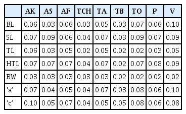
Variables were either positively or negatively correlated in both juveniles and male M. incognita populations (Table 3). Within the male populations, there was strong positive correlation between body length and greatest body width (r = 0.79), gubernaculum length and ‘c’ (r = 0.57), spicule length and gubernaculum length (r = 0.55), and body length and gubernaculum length (r = 0.54) in decreasing order of correlation strength (Table 3). There was also a strong negative correlation between greatest body width and ‘a’ (r = −0.98), tail length and ‘c’ (r = −0.92), and body length and ‘c’ (−0.66) also in decreasing order of strength (Table 3). Among the juvenile populations, strong positive correlations were between body length and ‘a’ (r = 0.91), body length and ‘c’ (r = 0.78), and ‘a’ and ‘c’ (r = 0.72) in decreasing order of correlation strength. A low negative correlation between greatest body width and ‘c’ (r = −0.35) and tail length and ‘c’ (r = −0.48) existed (Table 3).
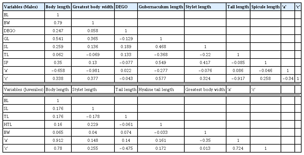
Pearson Correlation among variables for male and second-stage juvenile (J2) M. incognita populations
Correlations between variables and principal components
Variates were either positively or negatively correlated with the components in both juvenile and male M. incognita populations (Table 4). Highly correlated variables (positive) were greatest body width (r = 0.79), body length (r = 0.79), ‘c’ (r = 0.76) and gubernaculum length (r = 0.77), with PC1 and tail length (r = 0.70) with PC2 within the male M. incognita populations. The juvenile populations however, had body length (r = 0.92), ‘a’ (r = 0.92) and ‘c’ (r = 0.90) highly correlated with PC1, and tail length (r = 0.87) with PC2. Negatively correlated variables, tail length (r = −0.46) and a (r = −0.72) with PC1 and ‘a’ (r = −0.55) with PC2 within the male M. incognita. There were however no highly negatively correlated variables for juvenile M. incognita populations.
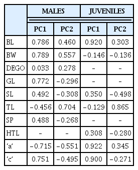
Correlations between variables and principal components (PC) for male and second-stage juvenile (J2) populations
Principal component analysis (PCA) of males and second-stage juveniles of M. incognita
A plot of PC1 and PC2 for M. incognita male populations showed clustering into three main groups (Fig. 1). Populations from Asuosu and Afrancho (Group I) were more closely related compared to populations from Tuobodom and Vea (Group II) (Fig. 1). There was however a single nematode from Afrancho (AF4) that fell into Group III. Biplots for male populations indicate, body length, DEGO, greatest body width, and gubernaculum length serving as variables distinguishing Group 1 and Group 2 populations. These same groupings from the PCA were reflected in the dendogram generated using Agglomerative Hierarchical Clustering (AHC) (Fig. 2).

Biplot for nine second-stage juvenile (J2) Meloidogyne incognita populations for PCA 1 and 2. Afrancho (AF), Akumadan (AK), Asuosu (AS), Toubodom (TB), Techimantia (TCH), Tanoso (TA), Tono (TO), Pwalugu (P) and Vea (V). 0–10 = Number of second-stage juvenile (J2) Meloidogyne incognita morphometrically characterised from each community. Color codings/groupings: Brown-Group 1 (Gp1), Violet-Group 2 (Gp2), and Green-Group 3(Gp3). Body length (BL), greatest body width (BW), stylet length (SL), tail length (TL), Hyaline tail length (HTL), ‘a’ = (total body length/greatest body width) and ‘c’ = (total body length/tail length).
Agglomerative Hierarchical Clustering (AHC) for nine second-stage juvenile (J2) Meloidogyne incognita populations. Afrancho (AF), Akumadan (AK), Asuosu (AS), Toubodom (TB), Techimantia (TCH), Tanoso (TA), Tono (TO), Pwalugu (P) and Vea (V). 0–10 = Number of second-stage juvenile (J2) Meloidogyne incognita morphometrically characterised from each community. Color codings/groupings: Brown-Group 1 (Gp1), Violet-Group 2 (Gp2), and Green-Group 3 (Gp3).
Within the M. incognita juvenile populations, although the plot of PC1 and PC2 revealed clustering of nematodes into three groups, there was overlap among these populations (Fig. 3). These was also evident in the dendogram generated using Agglomerative Hierarchical Clustering (AHC) (Fig. 4).
Biplot for four male Meloidogyne incognita populations for PCA 1 and 2. Asuosu (AS), Afrancho (AF), Toubodom (TB), and Vea (V). 0–4 = Number of male Meloidogyne incognita morphometrically characterised from each community. Color codings/groupings: Green-Group 1 (Gp1), Brown-Group 2 (Gp2), and Violet-Group 3(Gp3). Body length (BL), greatest body width (BW), Dorsal esophageal gland orifice (DEGO), gubernaculum length (GL), stylet length (SL), tail length (TL), spicule length (SP), ‘a’ = (total body length/greatest body width) and ‘c’ = (total body length/tail length).

Agglomerative Hierarchical Clustering (AHC) for four male Meloidogyne incognita populations. Asuosu (AS), Afrancho (AF), Toubodom (TB), and Vea (V). 0–4 = Number of male Meloidogyne incognita morphometrically characterised from each community. Color codings/groupings: Green-Group 1 (Gp1), Brown-Group 2 (Gp2), and Violet-Group 3 (Gp3).
Coefficient of variation
Coefficient of variation (CV) values for the various variables ranged from 0.02 to 0.10 for juveniles (Table 5). Variable with the least CV (0.02) were observed on greatest body width for Tuobodom, Tono, Pwalugu, and Vea populations. Variables with the largest CV values (0.10) were noted on body length and ‘a’ for Vea population, and ‘c’ for Akumadan population. The Vea and Techimantia populations had the highest (0.02–0.10) and lowest (0.03–0.04) ranges of CV values. Body length, hyaline tail length, and ‘a’ were the variables with the highest range (0.03–0.10) of CV values. Within the male populations, coefficient of variation (CV) ranged from 0.00 to 0.06 (Table 6). Variable with the least CV (0.00) were observed on body length for Asuosu, Afrancho, Tuobodom, and Vea populations, the greatest body width, Spicule length for Vea population, and Gubernaculum length for Asuosu population. Variables with the largest CV values (0.06) were noted on DEGO for Tuobodom and Vea populations. The Vea and Tuobodom populations had the highest ranges (0.00–0.06) of CV values.
Coefficient of variation for nine M. incognita second-stage juvenile (J2) populations from Ghana

Coefficient of variation for four M. incognita male populations from Ghana
Mean and standard deviation values for second-stage juvenile populations
Seven variables used in mean and standard deviation estimations for the juvenile populations revealed significant variability among them (Table 7). Body length measurements ranged from 320.01 μm to 440.27 μm. The highest standard deviation values were observed in body length, and these ranged from 14.27 to 38.24 for populations from Akumadan and Vea respectively.
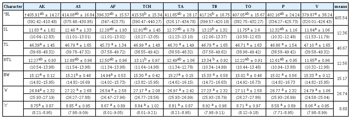
Mean and standard deviation values, and ranges for nine M. incognita (J2) populations from Ghana
There were no significant differences (p ≤ 0.05) for greatest body width, ‘a’ and ‘c’ in the juvenile populations. Average tail length in all the populations of M. incognita juveniles was 46.67 μm. The populations with the shortest (45.73 μm) and longest (47.10 μm) mean tail lengths were from Afrancho and Vea populations respectively.
Average hyaline tail terminus length for all the populations of M. incognita juveniles was 12.56 μm. The Vea population had the shortest hyaline tail terminus (11.65 μm) whiles the longest hyaline tail terminus came from the Techimantia population (13.34 μm).
Mean values for male populations
The mean and standard deviation values from the nine variables for male populations revealed significant variabilities among them (Table 8). There were significant differences (p ≤ 0.05) for Body length, greatest body width, gubernaculum length, spicule length and ‘a’. Afrancho population recorded the highest mean values for body length, gubernaculum length and spicule length.
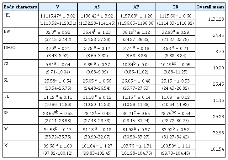
Mean and standard deviation values and ranges for four M. incognita male populations from Ghana
There were no significant differences (p ≤ 0.05) for DEGO, stylet length, tail length and ‘c’ in the populations, however, the Afrancho population had the highest mean values (26.05 μm, and 103.76 μm) for stylet length and ‘c’ respectively. This population further had the lowest mean value for tail length (45.73 μm). The longest tail lengths came from the Vea population (47.10 μm).
Body length measurements ranged from 1113.52 μm to 1196.86 μm, with the population from Afrancho having the longest mean body lengths (1157.63).
Gubernaculum length measurements ranged from 9.68 μm to 11.25 μm. The population from Afrancho had the longest length (10.84 μm) for gubernaculum length.
The highest standard deviation values were observed in the nematode body length and these ranged from 3.02 μm to 3.92 μm for Vea and Asuosu populations respectively.
Discussion
Principal Component Analysis (PCA) was used in grouping and distinguishing among nine populations of M. incognita juveniles and four populations of M. incognita males. This analysis is a multivariate technique for examining relationships among several quantitative variables and allows for the detection of linear relationships. Multivariate analysis was chosen because it represents an appropriate tool to assess distinctness and relationships between even closely related taxa or populations (Gould and Johnston, 1972; Reyment et al., 1981).
Although male M. incognita populations clustered into three groups, only a single nematode from Afrancho fell into Group III (AF4). This nematode had the highest values for body width (37.54) and spicule length (31.28). Populations from Asuosu and Afrancho (Group I) distinctly clustered from Tuobodom and Vea (Group II) populations. The group II populations did not have any significant differences among body length, maximum body width, ‘a’, and spicule length. Additional variables of importance are ‘c’, gubernaculum length, and tail length which had high positive correlations with PC1 and PC1 respectively. These variables will therefore be useful in distinguishing among M. incognita male populations. The juvenile populations also although were clustered into three groups at a dissimilarity value of 65, could be clustered into more than 10 sub-groups at a dissimilarity value less than 15. This is because of similarities in the variable measurements explaining the presence of variability among the populations. Body length, ‘a’, ‘c’, and tail length were highly correlated with PC1 and PC2 respectively among the juvenile populations. These variables are therefore important in identification of similarities in these populations.
Coefficient of variation (CV) values were low and these ranged from 0% to 10% for all the populations. A study by Nyaku et al. (2016), on reniform nematode population characterisation revealed variables with 5% to 15% CV. These variables were used in principal component analysis to distinguish among populations.
Correlations among the variables were either positive or negative for both males and juveniles. There were often overlaps in the measurements among male populations. Reports made previously on male M. incognita body lengths ranged from 1408 μm to 1792 μm (Jepson, 1983), and 1400 μm to 1780 μm (Zeng et al., 2014). A comparison of morphometric measurements of male M. incognita from Fiji by Singh (2009) revealed high variability among the nematodes, as was observed in our study. Longer body lengths of M. incognita have been reported (Singh, 2009). Measurements in our study were of lesser lengths, and the Afrancho population had the greatest variation in body lengths.
Reports made previously of juveniles ranged from 359.3 μm to 400 μm (Jepson, 1983), and 412 μm to 466 μm (Zeng et al., 2014). Shorter lengths ranging from 200 μm to 380 μm have also been made (Kaur and Attri, 2013). Average body lengths in our study were over 400 μm with the exception of populations from Afrancho and Vea, that had slightly lower values. This study provides the first report on morphometric characterisation of M. incognita male and juvenile populations in Ghana. Significant morphological variation exists among the juvenile populations compared to the male populations, because of the presence of sub-groups. The male M. incognita populations distinctly clustered into three groups. Variables of importance in distinguishing among the male populations are ‘c’ gubernaculum length and tail length.
Acknowledgments
The authors express profound gratitude to the A.G. Leventis Foundation, University of Ghana for financial support of this study.